Problem Statement: Design of a Thermal Fin

We consider the problem of designing a thermal fin(散热片) to effectively remove heat from a surface. The two-dimensional fin, shown in Figure 1, consists of a vertical central “post” and four horizontal “subfins”; the fin conducts heat from a prescribed uniform flux “source” at the root, $\Gamma_{\text{root}}$, through the large-surface-area subfins to surrounding flowing air.

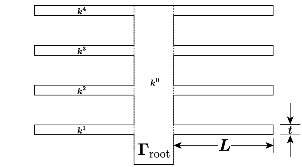
Figure 1: Thermal Fin

The fin is characterized by a five-component parameter vector, or “input,” $\underline{\mu}=(\mu^1,\mu^2,\mu^3,\mu^4,\mu^5)$ where $\mu^i=k^i, i=1,2,3,4$, and $\mu^5=\mathrm{Bi}$; $\underline{\mu}$ may take on any value in a specified design set $\mathcal{D}\subset\mathbb{R}^5$. Here $k^i$ is the thermal conductivity of the $i$th subfin (normalized relative to the post conductivity $k^0\equiv 1$); and $\mathrm{Bi}$ is the Biot number, a nondimensional heat transfer coefficient reflecting convective transport to the air at the fin surfaces (larger $\mathrm{Bi}$ means better heat transfer). For example, suppose we choose a thermal fin with $k^1=0.4$, $k^2=0.6$, $k^3=0.8$, $k^4=1.2$ and $\mathrm{Bi}=0.1$; for this particular configuration $\underline{\mu}=\lbrace0.4, 0.6, 0.8, 1.2, 0.1\rbrace$, which corresponds to a single point in the set of all possible configurations $\mathcal{D}$ (the parameter or design set). The post is of width unity and height four; the subfins are of fixed thickness $t = 0.25$ and length $L = 2.5$.

We are interested in the design of this thermal fin, and we thus need to look at certain outputs or cost-functionals of the temperature as a function of $\underline{\mu}$. We choose for our output $T_{\text{root}}$, the average steady-state temperature of the fin root normalized by the prescribed heat flux into the fin root. The particular output chosen relates directly to the cooling efficiency of the fin — lower values of $T_{\text{root}}$ imply better thermal performance.

The steady-state temperature distribution within the fin, $u(\underline{\mu})$, is governed by the elliptic partial differential equation

\[-k^i\nabla^2u^i=0\text{ in }\Omega^i, \quad i=0,1,2,3,4,\]

where $\nabla^2$ is the Laplacian operator, and $u^i$ refers to the restriction of $u$ to $\Omega^i$. Here $\Omega^i$ is the region of the fin with conductivity $k^i, i=0,1,2,3,4$; $\Omega^0$ is thus the central post, and $\Omega^i, i=1,2,3,4,$ corresponds to the four subfins. The entire fin domain is denoted $\Omega$ ($\overline{\Omega}=\bigcup_{i=0}^4\overline{\Omega^i}$); the boundary of $\Omega$ is denoted $\Gamma$. We must also ensure continuity of temperature and heat flux at the conductivity-discontinuity interfaces $\Gamma_{\mathrm{int}}^i\equiv\partial\Omega^0\cap\partial\Omega^i, i=1,2,3,4$, where $\partial\Omega^i$ denotes the boundary of $\Omega^i$:

\[\left.\begin{aligned} u^0&=u^i \\ -(\nabla u^0\cdot\hat{\mathbf{n}}^i)&=-k^i(\nabla u^i\cdot\hat{\mathbf{n}}^i) \end{aligned}\right\}\text{ on }\Gamma_{\text{int}}^i, \quad i=1,2,3,4.\]

here $\hat{\mathbf{n}}^i$ is the outward normal on $\partial\Omega^i$. Finally, we introduce a Neumann flux boundary condition on the fin root

\[-(\nabla u^0\cdot\hat{\mathbf{n}}^0)=-1\text{ on }\Gamma_{\text{root}},\]

which models the heat source; and a Robin boundary condition

\[-k^i(\nabla u^i\cdot\hat{\mathbf{n}}^i)=\mathrm{Bi}\,\, u^i\text{ on }\Gamma_{\text{ext}}^i, i=0,1,2,3,4,\]

which models the convective heat losses. Here $\Gamma_{\text{ext}}^i$ is that part of the boundary of $\Omega^i$ exposed to the flowing fluid; note that $\bigcup_{i=0}^4\Gamma_{\text{ext}}^i=\Gamma\setminus\Gamma_{\text{root}}.$

The average temparature at the root, $T_{\text{root}}(\underline{\mu})$, can then be expressed as $\ell^O(u(\underline{\mu}))$, where

\[\ell^O(v)=\int_{\Gamma_{\text{root}}}v\]

(recall $\Gamma_{\text{root}}$ is of length unity). Note that $\ell(v)=\ell^O(v)$ for this problem.

Part 1: Finite Element Approximation

(1)Show that $u(\underline{\mu})\in X\equiv H^1(\Omega)$ satisfies the weak form

\[a(u(\underline{\mu}),v; \underline{\mu})=\ell(v), \qquad \forall v\in X,\]

with

\[\begin{aligned} a(w,v;\underline{\mu}) & =\sum_{i=0}^4k^i\int_{\Omega^i}\nabla w\cdot\nabla v\mathrm{d}A +\mathrm{Bi}\int_{\Gamma\setminus\Gamma_{\text{root}}}wv\mathrm{d}S, \\ \ell(v)&=\int_{\Gamma_{\text{root}}}v\mathrm{d}S. \end{aligned}\]

(2)Show that $u(\underline{\mu})$ is the argument that minimizes

\[J(w)=\dfrac{1}{2}\sum_{i=0}^4k^i\int_{\Omega^i}\nabla w\cdot\nabla w\mathrm{d}A +\dfrac{\mathrm{Bi}}{2}\int_{\Gamma\setminus\Gamma_{\text{root}}}w^2\mathrm{d}S -\int_{\Gamma_{\text{root}}}w\mathrm{d}S\]

over all functions $w$ in $X$.

(3)We now consider the linear finite element space

\[X_h=\left\{v\in H^1(\Omega)\Big| v|_{T_h}\in \mathbb{P}^1(T_h), \forall T_h\in\mathcal{T}_h\right\},\]

and look for $u_h(\underline{\mu})\in X_h$ such that

\[a(u_h(\underline{\mu}), v; \underline{\mu})=\ell(v), \qquad \forall v\in X_h;\]

our output of interest is then given by

\[T_{\mathrm{root\,}h}(\underline{\mu})=\ell^O(u_h(\underline{\mu})).\]

Applying our usual nodal basis, we arrive at the matrix equations

\[\begin{aligned} \underline{A}_h\underline{u}_h(\underline{\mu})&=\underline{F}_h, \\ T_{\mathrm{root\,}h}(\underline{\mu})&=(\underline{L}_h)^T\underline{u}_h(\underline{\mu}), \end{aligned}\]

where $\underline{A}_h\in\mathbb{R}^{n\times n}$, $\underline{u}_h,\underline{F}_h,\underline{L}_h\in\mathbb{R}^n$; here $n$ is the dimension of the finite element space, which (given our natural boundary conditions) is equal to the number of nodes in $\mathcal{T}_h$.

Derive the elemental matrices $\underline{A}_h^k \in\mathbb{R}^{3\times3}$, load vectors $\underline{F}_h^k \in\mathbb{R}^{3}$, and output vectors, $\underline{L}_h^k \in\mathbb{R}^{3}$, with particular attention to those elements on $\Gamma$; and describe the procedure for creating $\underline{A}_h$, $\underline{F}_h$, and $\underline{L}_h$ from these elemental quantities.

(4)Write a finite-element code that takes a configuration $\underline{\mu}$ and a triangulation $\mathcal{T_{h}}$ (see Appendix 1), and returns $u_h(\underline{\mu})$ and $T_{\text{root } h}(\underline{\mu})$.

For the particular configuration $\underline{\mu_{0}}=\lbrace 0.4, 0.6, 0.8, 1.2, 0.1\rbrace$, (i) plot the solution $u_h(\underline{\mu_{0}})$ (see Appendix 1), and (ii) evaluate the output $T_{\text{root } h}(\underline{\mu_0})$; use $\mathcal{T_{h_{\text{medium}}}}$ for this calculation.

(5)Show that

\[T_{\text{root}}(\underline{\mu})-T_{\text{root } h}(\underline{\mu}) =a(e(\underline{\mu}),e(\underline{\mu})),\]

where $e(\underline{\mu})=u(\underline{\mu})-u_h(\underline{\mu})$ is the error in the finite element solution. If $u\in H^2(\Omega)$, how would you expect $T_{\text{root}}(\underline{\mu})-T_{\text{root } h}(\underline{\mu})$ to converge as a function of $h$? In practice, what do you observe? To answer the latter question, take the finest of the three triangulations given $(\mathcal{T_{h_{\text{fine}}}})$ as the “truth,” and suppose that

\[\begin{aligned} (T_{\text{root}}(\underline{\mu}))_{h_{\text{fine}}}-(T_{\text{root}}(\underline{\mu}))_{2h_{\text{fine}} =h_{\text{medium}}} &=C(2h_{\text{fine}})^b \\ (T_{\text{root}}(\underline{\mu}))_{h_{\text{fine}}}-(T_{\text{root}}(\underline{\mu}))_{4h_{\text{fine}} =h_{\text{coarse}}} &=C(4h_{\text{fine}})^b \end{aligned}\]

then find $b$ in the obvious fashion.