完成日期:2022年10月16日
Table of Contents
Problem Formulation
Consider the following differential equation
\[\begin{aligned} -\dfrac{\mathrm{d}^2u}{\mathrm{d}x^2}+\dfrac{\mathrm{d}u}{\mathrm{d}x}+u&=f(x), &&x\in\Omega=(0,1), \\ u(0)&=0, \\ u(1)&=1, \end{aligned}\]where $f(x)=(\frac{1}{4}\pi^2+1)\sin(\frac{1}{2}\pi x)+\frac{1}{2}\pi\cos(\frac{1}{2}\pi x)$. The exact solution for this problem is given by $u(x)=\sin(\frac{1}{2}\pi x).$
1. Show that the weak formulation can be written as
\[a(u,v)=F(v), \qquad \forall v\in V,\]where $V=\lbrace v\in L^2(\Omega): v’\in L^2(\Omega)\text{ and }v(0)=v(1)=0\rbrace$, $G$ is some appropriate function, and
\[\begin{aligned} a(u,v)&=\int_{\Omega}(u'v'+u'v+uv)\mathrm{d}x, \\ F(v)&=\int_{\Omega}fv\mathrm{d}x-\int_{\Omega}(G'v'+G'v+Gv)\mathrm{d}x, \end{aligned}\]2. Implement the finite element method on a uniform grid with mesh points $0 = x_0 < x_1 < \cdots < x_N=1$ where $x_j=jh$, $h=1/N$ is the element size, and $N$ is the number of elements. Note that the basis for $V_h\subset V$ is $\lbrace \phi_1,\cdots,\phi_{N-1}\rbrace$.
3. Plot the solution on a grid with $N=8$ elements. Compute the error in the $L^2(\Omega)$-norm for $N=8,16,32,64,128,256$ and 512 elements. Compute at what rate $r$ the error decreases.
Solution
Problem 1
(1)Let $G(x)$ satisfy $G(0)=0$, $G(1)=-1$, and
\[-\dfrac{\mathrm{d}^2G}{\mathrm{d}x^2}+\dfrac{\mathrm{d}G}{\mathrm{d}x}+G=0. \tag{1}\]This is an ODE with characteristic equation
\[\lambda^2-\lambda-1=0,\]the solution of which is $\lambda_1=\dfrac{1+\sqrt{5}}{2}$ and $\lambda_2=\dfrac{1-\sqrt{5}}{2}.$ So
\[G(x)=C_1e^{\lambda_1x}+C_2e^{\lambda_2x}.\]From $G(0)=0$, $G(1)=-1$, we have
\[\left\{\begin{aligned} &0=C_1+C_2, \\ &-1 =C_1e^{\lambda_1}+C_2e^{\lambda_2}, \end{aligned}\right. \Rightarrow \left\{\begin{aligned} &C_1=-\dfrac{1}{e^{\lambda_1}-e^{\lambda_2}} , \\ &C_2=\dfrac{1}{e^{\lambda_1}-e^{\lambda_2}}. \end{aligned}\right.\]So $G(x)=-\dfrac{e^{\lambda_1x}-e^{\lambda_2x}}{e^{\lambda_1}-e^{\lambda_2}}$ satisfies $G(0)=0$ and $G(1)=-1$ and $(1)$.
(2)Now consider $w=u+G$. Then
\[\left\{\begin{aligned} &-\dfrac{\mathrm{d}^2w}{\mathrm{d}x^2}+\dfrac{\mathrm{d}w}{\mathrm{d}x}+w=f, && \text{ in }(0,1), \\ &w(0)=0, \\ &w(1)=0. \end{aligned}\right.\]For any $v\in V$, multiplying both sides of the above PDE by $v$, and using integration by parts, we have
\[\begin{aligned} \int_{\Omega}fv\mathrm{d}x&=\int_{\Omega}\left(-\dfrac{\mathrm{d}^2w}{\mathrm{d}x^2} +\dfrac{\mathrm{d}w}{\mathrm{d}x}+w\right)v\mathrm{d}x \\ &=\int_{\Omega}w'v'\mathrm{d}x-w'v'\Big|_0^1+\int_{\Omega}(w'v+wv)\mathrm{d}x \\ &=\int_{\Omega}(w'v'+w'v+wv)\mathrm{d}x \\ &=\int_{\Omega}(u'v'+u'v+uv)\mathrm{d}x+\int_{\Omega}(G'v'+G'v+Gv)\mathrm{d}x. \end{aligned}\]Thus, the weak formulation is
\[a(u,v)=F(v),\]where $a(u,v)$ and $F(v)$ satisfy
\[\begin{aligned} a(u,v)&=\int_{\Omega}(u'v'+u'v+uv)\mathrm{d}x, \\ F(v)&=\int_{\Omega}fv\mathrm{d}x-\int_{\Omega}(G'v'+G'v+Gv)\mathrm{d}x, \end{aligned}\]The Galerkin method is:
\[\text{Find $u_h\in V_h$ such that $a(u_h,v_h)=F(v_h), \forall v_h\in V_h.$} \tag{2}\]Problem 2
Construction of stiffness matrix and load vector
Note that $(2)$ is equivalent to
\[\text{Find $w_h\in V_h$ such that $a(w_h,v_h)=\int_{\Omega}fv_h\mathrm{d}x, \forall v_h\in V_h.$} \tag{3}\]Now, for $V_h=\mathrm{span}\lbrace\phi_1,\cdots,\phi_{N-1}\rbrace$, denote
\[w_h=\sum_{j=1}^{N-1}w_j\phi_j, \qquad w_j\in\mathbb{R},\]Then, $u_h=\sum\limits_{j=1}^{N-1}(w_j-g_j)\phi_j$(where $g_j=G(x_j)$) is the solution of $(2)$. So we only need to solve $(3)$.
For $v_h=\phi_i, i=1,\cdots,N-1$, we have
\[a(w_h,\phi_i)=\sum_{j=1}^{N-1}w_j\int_{\Omega}(\phi_j'\phi_i'+\phi_j'\phi_i+\phi_j\phi_i)\mathrm{d}x =\sum_{j=1}^{N-1}w_ja(\phi_j,\phi_i)\]and
\[F(\phi_i)=\int_{\Omega}f\phi_i\mathrm{d}x.\]Now take
\[\begin{aligned} &A=[a_{ij}], \text{ where }a_{ij}=a(\phi_j,\phi_i), \\ &W=[w_1,\cdots,w_{N-1}]^T\in\mathbb{R}^{N-1}, \\ &F=[F(\phi_1),\cdots,F(\phi_{N-1})]^T\in\mathbb{R}^{N-1}. \end{aligned}\]Then we have the following matrix form of $(2)$:
\[AW=F. \tag{4}\]It remains to calculate the components of $A$ and $F$. Consider the nodal basis
\[\phi_j(x)=\left\{\begin{aligned} &\dfrac{x-x_{j-1}}{h}, && \text{ in }[x_{j-1},x_j], \\ &\dfrac{x_{j+1}-x}{h}, && \text{ in }[x_j,x_{j+1}], \\ &0, && \text{ otherwise}. \end{aligned}\right.\]The support of $\phi_j$ is $\mathrm{supp}(\phi_j)=[x_{j-1},x_{j+1}]$. From
\[a_{ij}=a(\phi_j,\phi_i)=\int_{\Omega}(\phi_j'\phi_i'+\phi_j'\phi_i+\phi_j\phi_i)\mathrm{d}x,\]it is easy to see that
\[a_{ij}=0 \text{ if } |i-j|\ge 2.\]Moreover, $\mathrm{supp}(\phi_{j-1})\cap\mathrm{supp}(\phi_j)=[x_{j-2},x_j]\cap[x_{j-1},x_{j+1}] =[x_{j-1},x_j]$, so
\[\begin{aligned} a_{j-1,j}&=\int_{x_{j-1}}^{x_j}\left(-\dfrac{1}{h}\cdot\dfrac{1}{h}+\dfrac{1}{h}\cdot\dfrac{x_j-x}{h} +\dfrac{x-x_{j-1}}{h}\cdot\dfrac{x_j-x}{h}\right)\mathrm{d}x \\ &=\dfrac{1}{h^2}\left(-h+\dfrac{1}{2}h^2+\dfrac{1}{6}h^3\right) \\ &=\dfrac{h}{6}+\dfrac{1}{2}-\dfrac{1}{h}. \end{aligned}\]Similarly,
\[\begin{aligned} a_{j+1,j}&=\int_{x_{j}}^{x_{j+1}}\left(-\dfrac{1}{h}\cdot\dfrac{1}{h}+\dfrac{1}{h}\cdot\dfrac{x-x_j}{h} +\dfrac{x_{j+1}-x}{h}\cdot\dfrac{x-x_j}{h}\right)\mathrm{d}x \\ &=\dfrac{1}{h^2}\left(-h-\dfrac{1}{2}h^2+\dfrac{1}{6}h^3\right) \\ &=\dfrac{h}{6}-\dfrac{1}{2}-\dfrac{1}{h}. \end{aligned}\]and
\[\begin{aligned} a_{j,j}&=\int_{x_{j-1}}^{x_j}\left(\dfrac{1}{h^2}+\dfrac{1}{h}\cdot\dfrac{x-x_{j-1}}{h} +\dfrac{(x-x_{j-1})^2}{h^2}\right)\mathrm{d}x \\ &\qquad +\int_{x_{j}}^{x_{j+1}}\left(\dfrac{1}{h^2}-\dfrac{1}{h}\cdot\dfrac{x_{j+1}-x}{h} +\dfrac{(x_{j+1}-x)^2}{h^2}\right)\mathrm{d}x \\ &=\dfrac{1}{h^2}\left(h+\dfrac{1}{2}h^2+\dfrac{1}{3}h^3\right) +\dfrac{1}{h^2}\left(h-\dfrac{1}{2}h^2+\dfrac{1}{3}h^3\right) \\ &=\dfrac{1}{h^2}\left(2h+\dfrac{2}{3}h^3\right)=\dfrac{2h}{3}+\dfrac{2}{h}. \end{aligned}\]Finally, by some long and boring calculation,
\[\begin{aligned} \int_{\Omega}f\phi_i\mathrm{d}x &=\dfrac{8}{\pi^2h}\left(\dfrac{1}{4}\pi^2+1\right)\sin\left(\dfrac{\pi x_i}{2}\right) +\dfrac{4}{\pi h}\cos\left(\dfrac{\pi x_i}{2}\right) \\ &\qquad -\dfrac{4}{\pi^2h}\left(\dfrac{1}{4}\pi^2+1\right)\sin\left(\dfrac{\pi x_{i-1}}{2}\right) -\dfrac{2}{\pi h}\cos\left(\dfrac{\pi x_{i-1}}{2}\right) \\ &\qquad -\dfrac{4}{\pi^2h}\left(\dfrac{1}{4}\pi^2+1\right)\sin\left(\dfrac{\pi x_{i+1}}{2}\right) -\dfrac{2}{\pi h}\cos\left(\dfrac{\pi x_{i+1}}{2}\right) . \end{aligned}\]We can now use Matlab to solve equation $(3)$. After that, take
\[\tilde{G}=(g_1,g_2,\cdots,g_{N-1})^T\in\mathbb{R}^{N-1}\]and let
\[U=W-\tilde{G},\]then $U$ is the FEM solution of $(4)$.
Matlab Code
N = 8;
h = 1.0/N;
x = 0:h:1; %x(i)=x_{i-1}
u_real = sin(pi*x/2);

%% Stiffness matrix
a1 = -1.0/h-1.0/2+h/6; %a_{j+1,j}
a2 = 2.0/h+2.0*h/3; %a_{j,j}
a3 = -1.0/h+1.0/2+h/6; %a_{j-1,j}
e = ones(N-1,1);
A = spdiags([a1*e a2*e a3*e],-1:1,N-1,N-1);
% spy(A) %print A as a graph
% full(A) %print A

%% Load vector
F = zeros(N-1,1);
for i = 1:N-1
    F(i)=-(1.0/h+4.0/pi/pi/h)*(sin(pi*x(i)/2)+sin(pi*x(i+2)/2)-2*sin(pi*x(i+1)/2)) ...
          -2.0/pi/h*(cos(pi*x(i)/2)+cos(pi*x(i+2)/2)-2*cos(pi*x(i+1)/2));
end
W = A\F;

%% G
lam1 = (1+sqrt(5))/2;
lam2 = (1-sqrt(5))/2;
G = -(exp(lam1*x)-exp(lam2*x))/(exp(lam1)-exp(lam2));
%G = zeros(N-1,1);
%for i = 1:N-1
%    G(i)=-(exp(lam1*x(i+1))-exp(lam2*x(i+1)))/(exp(lam1)-exp(lam2));
%end

%% Plotting
U = [0 W' 0] - G;
%plot(x,UU,'--r',x,u_real,'-b'); %Plot FEM solution and real solution
%legend('FEM solution','real solution','location','northwest');
plot(x,U,'r-o');
legend('FEM solution','location','northwest');
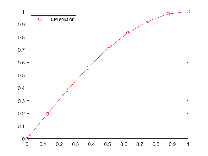
Figure 1: Solution of $n=8$.
Problem 3
Matlab Code
Ns = [8,16,32,64,128,256,512];
%Ns = [8];
errs = zeros(7,1);
for m = 1:7
    N = Ns(m);
    h = 1.0/N;
    x = 0:h:1; %x(i)=x_{i-1}
    u_real = sin(pi*x/2);

    %% Stiffness matrix
    a1 = -1.0/h-1.0/2+h/6; %a_{j+1,j}
    a2 = 2.0/h+2.0*h/3; %a_{j,j}
    a3 = -1.0/h+1.0/2+h/6; %a_{j-1,j}
    e = ones(N-1,1);
    A = spdiags([a1*e a2*e a3*e],-1:1,N-1,N-1);
    % spy(A) %print A as a graph
    % full(A) %print A

    %% Load vector
    F = zeros(N-1,1);
    for i = 1:N-1
        F(i)=-(1.0/h+4.0/pi/pi/h)*(sin(pi*x(i)/2)+sin(pi*x(i+2)/2)-2*sin(pi*x(i+1)/2)) ...
              -2.0/pi/h*(cos(pi*x(i)/2)+cos(pi*x(i+2)/2)-2*cos(pi*x(i+1)/2));
    end
    W = A\F;

    %% G
    lam1 = (1+sqrt(5))/2;
    lam2 = (1-sqrt(5))/2;
    G = -(exp(lam1*x)-exp(lam2*x))/(exp(lam1)-exp(lam2));

    U = [0 W' 0] - G;

    %% Computing L2 Error
    err = 0;
    for i = 1:N
        %Get x from [x_{i-1},x_i]
        points = 50;
        d = (x(i+1)-x(i))/points;
        xx = x(i):d:x(i+1);
        %Get U between U_{i-1} and U_{i}
        p = polyfit([x(i),x(i+1)],[U(i),U(i+1)],1);
        uu = polyval(p,xx);
        uu_real = sin(pi*xx/2);
        %Calculate square of L2 error
        err = err + norm(uu-uu_real)^2;
    end
    err = sqrt(err)/(points+1); %need to take a root because err is squared
    errs(m) = err; %store error into array errs
end

%% Compute the rate r the error decreases.
%err = Ch^{r}, so log err = log C+rlog h.
%So we need to find a relation between log h and log err.

hh = log(1./Ns);
logerr = log(errs);
plot(hh,logerr);
xlabel("log h");
ylabel('log err');
legend('logerr');
err_fit = polyfit(hh,logerr,1);
% log err = r log h + log C,
% r=err_fit(1) represents the rate, log C=err_fit(2).

fprintf("The rate r the error decreases is %f \n", err_fit(1));
Output: The rate r the error decreases is 1.500822
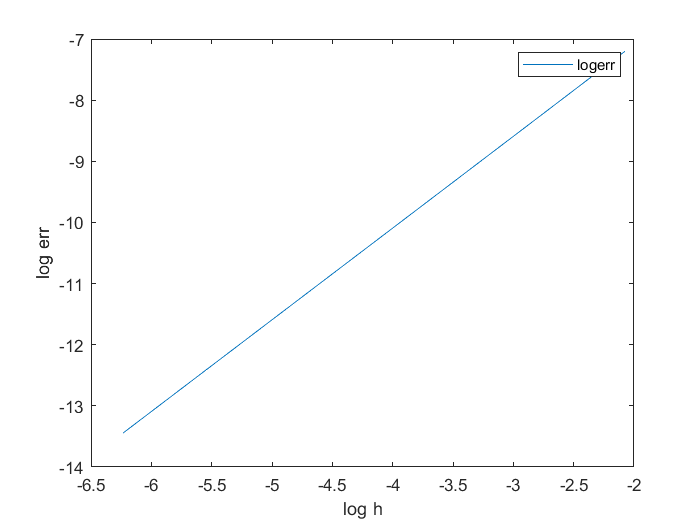
Figure 2: The fit curve of $\log err = r\log h+\log C$.