完成日期：2022年5月27日

出处：MIT, Numerical Methods for Partial Differential Equations

更多内容：http://lie.math.brocku.ca/~sanco/solitons/kdv_solitons.php

J. Scott Russell wrote in 1844:

“I believe I shall best introduce this phenomenon by describing the circumstances of my own first acquaintance with it. I was observing the motion of a boat which was rapidly drawn along a narrow channel by a pair of horses, when the boat suddenly stopped - not so the mass of water in the channel which it had put in motion; it accumulated round the prow of the vessel in a state of violent agitation, then suddenly leaving it behind, rolled forward with great velocity, assuming the form of a large solitary elevation, a rounded, smooth and well defined heap of water, which continued its course along the channel apparently without change of form or diminution of speed. I followed it on horseback, and overtook it still rolling on at a rate of some eight or nine miles an hour, preserving its original figure some thirty feet long and a foot to a foot and a half in height. Its height gradually diminished, and after a chase of one or two miles I lost it in the windings of the channel.”

Problem Statement

In 1895, Korteweg and de Vries formulated the equation

which models Russell’s observation. The term $uu_x$ describes the sharpening of the wave and $u_{xxx}$ the dispersion (i.e., waves with different wave lengths propagate with different velocities). The balance between these two terms allows for a propagating wave with unchanged form. The primary application of solitons today are in optical fibers, where the linear dispersion of the fiber provides smoothing of the wave, and the non-linear properties give the sharpening. The result is a very stable and long-lasting pulse that is free from dispersion, which is a problem with traditional optical communication techniques.

Questions

(1)Show using direct substitution that the one-soliton solution

solves the KdV equation (1). Here, $v>0$ and $x_0$ are arbitrary parameters.

(2)We will solve the KdV equation numerically using the method of lines and finite difference approximations for the space derivatives. Rewrite the equation as

and derive a second-order accurate difference approximation of the right-hand side.

(3)For the time integration, we will use a fourth order Runge-Kutta scheme:

The stability region for this scheme consists of all $z$ such that $\left|1+z+\dfrac{z^2}{2}+\dfrac{z^3}{6}+\dfrac{z^4}{24}\right| \le 1.$ In particular, all points on the imaginary axis between $\pm i2\sqrt{2}$ are included.

Our equation $(1)$ is non-linear, and to make a stability analysis we first have to linearize it. In this case, it turns out that the stability will be determined by the discretization of the third-derivative term $u_{xxx}$. Therefore, consider the simplified problem

and use von Neumann stability analysis to derive an expression for the maximum allowable time-step $\Delta t$ in terms of $\Delta x$.

(4)Write a program that solves the equation using your discretization. Solve it in the region $-8\le x\le 8$ with a grid size $\Delta x=0.1$, and use periodic boundary conditions:

Integrate from $t = 0$ to $t = 2$, using an appropriate time-step that satisfies the condition you derived above. For each of the initial conditions below, plot the solution at $t = 2$ and comment on the results.

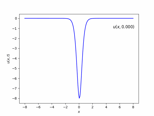
• a. To begin with, use a single soliton $(2)$ as initial condition, that is, $u(x,0)=u_1(x,0)$. Set $v=16$ and $x_0=0$.
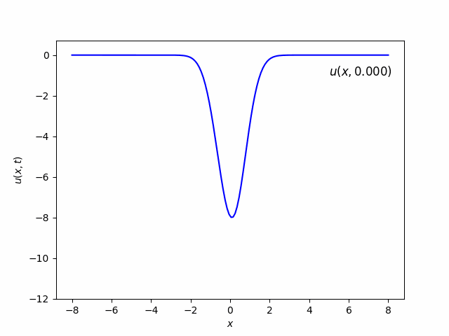
• b. The one-soliton solution looks almost like a Gaussian. Try $u(x,0)=-8e^{-x^2}$.
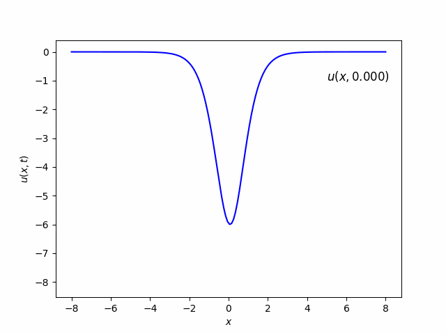
• c. Try the two-soliton solution $u(x,0)=-6/\cosh^2(x)$.
• d. Create “your own” two-soliton solution by superposing two one-soliton solutions with $v=16$ and $v=4$ (both with $x_0=0$).
• e. Same as before, but with $v = 16,x_0= 4$ and $v = 4,x_0= -4$. Describe what happens when the two solitons cross (amplitudes, velocities), and after they have crossed.

Solutions

Question 1

Question 1

Show using direct substitution that the one-soliton solution

\[u_1(x,t)=-\dfrac{v}{2\cosh^2\left(\frac{1}{2}\sqrt{v}(x-vt-x_0)\right)} \tag{2}\]

solves the KdV equation (1). Here, $v>0$ and $x_0$ are arbitrary parameters.

Question 2

Question 3

Question 4

Question 4

Write a program that solves the equation using your discretization. Solve it in the region $-8\le x\le 8$ with a grid size $\Delta x=0.1$, and use periodic boundary conditions:

\[x(-8)=x(8).\]

Integrate from $t = 0$ to $t = 2$, using an appropriate time-step that satisfies the condition you derived above. For each of the initial conditions below, plot the solution at $t = 2$ and comment on the results.

• a. To begin with, use a single soliton $(2)$ as initial condition, that is, $u(x,0)=u_1(x,0)$. Set $v=16$ and $x_0=0$.
• b. The one-soliton solution looks almost like a Gaussian. Try $u(x,0)=-8e^{-x^2}$.
• c. Try the two-soliton solution $u(x,0)=-6/\cosh^2(x)$.
• d. Create “your own” two-soliton solution by superposing two one-soliton solutions with $v=16$ and $v=4$ (both with $x_0=0$).
• e. Same as before, but with $v = 16,x_0= 4$ and $v = 4,x_0= -4$. Describe what happens when the two solitons cross (amplitudes, velocities), and after they have crossed.

Codes:

import numpy as np
import matplotlib.pyplot as plt
import matplotlib.animation as animation

a = -8
b = 8
dx = 0.1
n = 160 #int((b-a)/dx) #number of subintervals
xs = np.linspace(a,b,n)

# dt/(dx)^3<=sqrt(2), so we can take dt = 0.001.
dt = 0.001
T = 2

def KdV(u1, plot = False, fileName = 'KdV.gif'):
    def f(u): #u is a vector, len(u)=n. u[n]=x(8)=x(-8)=u[0].
        v = np.zeros(n)
        for i in range(n):
            i1 = (i+1)%n #u_i}
            i2 = (i+2)%n #u_{i+2}
            im1 = (i-1+n)%n # u_{i-1}
            im2 = (i-2+n)%n # u_{i-2}.To ensure periodic boundary.
            v[i] = 6*(u[i1]-u[im1])*u[i]/2.0/dx - (u[i2]-2*u[i1]+2*u[im1]-u[im2])/2.0/(dx**3)
        return v

    def RK4(u):# u is a vector
        k1 = dt*f(u)
        k2 = dt*f(u+k1/2.0)
        k3 = dt*f(u+k2/2.0)
        k4 = dt*f(u+k3)
        y = k1/6.0+k2/3.0+k3/3.0+k4/6.0 #RK4
        return y

    u = np.zeros(n)
    for i in range(n):
        u[i] = u1(a + i*dx, 0) #initial solution

    cnt = 0 #count
    t = 0
    if(plot):
        plt.cla()
        fig = plt.figure(10)
        ims = [] #Animation
        plt.xlabel(r'$x$')  
        plt.ylabel(r'$u(x,t)$')  
        
        while t<=T:
            u_tmp = u + RK4(u)
            u = u_tmp
            #plt.cla()
            #plt.pause(0.000001)
            if(cnt % 50 == 0):
                im = plt.plot(xs, u, c = 'b', label = '$u(x,{tt:.3f})$'.format(tt = t))
                im1 = plt.text(5,-1, '$u(x,{tt:.3f})$'.format(tt = t), fontsize = 12)
                ims.append(im + [im1])
                print(t)
            cnt = cnt + 1
            t = t + dt

        ani = animation.ArtistAnimation(fig, ims, interval=20, repeat_delay = 500)
        ani.save(fileName,writer='pillow', fps = 10)
    else:
        while t<=T:
            u_tmp = u + RK4(u)
            u = u_tmp
            t = t + dt
    return u

if __name__ == "__main__": 
    #Exercise a
    v = 16
    x0 = 0
    def u1(x,t):
        return (-v/2.0/(np.cosh(0.5*np.sqrt(v)*(x-v*t-x0))**2))
    u = KdV(u1, True, 'KdVa.gif')

    #Exercise b
    def u2(x,t):
        return (-8*np.exp(-x*x))
    u = KdV(u2, True, 'KdVb.gif')
    
    #Exercise c
    def u3(x,t):
        return (-6/(np.cosh(x)**2))
    u = KdV(u3, True, 'KdVc.gif')

Part (a)

In this case, there is one soliton which looks like Gaussian function and move from left to right as time goes.

Part (b) & (c)

In the beginning, it looks like there is only one soliton. But as time goes, it will be splitted into two solitons. The one with higher amplitude has more velocity than the one with lower amplitude.

Part (d) & (e)

We omit the results of (d) and (e).